Tag: R

283 tweets about flu today

I wanted to use the TwitteR package for R since a long time, I tried but didn’t do much of it. Today I found a few minutes, followed simple recipes (I admit), and looked at the number of tweets about flu today (November 13, 2018). Result: 283 tweets in English (I wanted to focus on the USA but, for some reason, I couldn’t … yet!). That’s not a lot. But remember we are only at the beginning of the influenza season 2018-2019 in the Northern hemisphere.

After some very basic cleaning, here are the words most used: flu, influenza (obviously: I was looking for them!), rt (note to self: remove this indication of a retweet), vaccine, health and get. As I mentioned: we are at the beginning of the flu season in the Northern hemisphere, it’s still time to get vaccinated and protected against flu!

1811130-wordFreq

Now of course, I wanted a word cloud 😉 Here it is:

181113-wordcloud

It’s basically the same graph as above. You don’t get the count but you get the feeling of how important each word is (and you get more words).

I also recently read the recent WIRED article about the need of less stats and more stories about the success of vaccines. And I was wondering if, by following tweets and people on Twitter, tweeting about flu, we could reconstruct stories about influenza and vaccination against it. I’ll try to dedicate a few minutes every now and then, during this season, to this. In the meantime, if you have additional ideas, don’t hesitate to send them to me, comment below, or contact me … on Twitter, obviously! (I’m @jepoirrier)

More sleep with Fitbits

After a bit less than 2 hours, jepsfitbitapp retrieved my sleep data from Fitbit for the whole 2013 (read previous post for the why (*)). Since this dataset covers the period I didn’t have a tracking device and, more broadly, I always slept at least a little bit at night, I removed all data point where it indicates I didn’t sleep.

hours alseep with FitbitSo I slept 5 hours and 37 minutes on average in 2013 with one very short night of 92 minutes and one very nice night of 12 hours and 44 minutes. Fitbits devices do not detect when you go to sleep and when you wake up: you have to tell tem (for instance by tapping 5 times on the Flex) that you go to sleep or you wake up (by the way this is a very clever way to use the Flex that has no button). Once told you are in bed the Flex manages to determine the number of minutes to fall asleep, after wakeup, asleep, awake, … The duration mentioned here is the real duration the Fitbit device considers I sleep (variable minutesAsleep).

Visually it looks like there is a tendency to sleep more as 2013 passes. But, although the best linear fit shows an angle, the difference between sleep in March and sleep in December is not significant.

R allows to study the data in many different ways (of course!). When plotting the distribution of durations asleep it seems this may be distributed like a normal (Gaussian) distribution (see the graph below). But the Shapiro-wilk normality test shows that the data doesn’t belong to a normal distribution.

Histogram of hours asleep in 2013Hours asleep in 2013 - Normal?As mentioned above, Fitbit devices are tracking other sleep parameters. Among them there is the number of awakenings and the sleep efficiency.

Awakenings in 2013

The simple plot of the number of awakenings over time shows the same non-significant trend as the sleep duration (above). The histogram of these awakenings shows a more skewed distribution to the left (to a low number of awakenings) (than the sleep duration). This however shows there is a relation between the two variables: the more I sleep the more the Flex detects awakenings (see second graph below).

Number of awakenings in 2013 (histogram)Relation between sleep duration and awakenings with Fitbit FlexSleep efficiency is the ratio between the total time asleep by the total time in bed from the moment I fell asleep. This is therefore not something related to the different sleep stages. However it may indicate an issue worth investigating with a real doctor. In my case, although I woke up 9 time per night on average in 2013, my sleep efficiency is very high (93.7% on average) …

Sleep efficiency in 2013… or very low. There are indeed some nights where my sleep efficiency is below 10% (see the 4 points at the bottom of the chart). These correspond with nights when I didn’t sleep a lot and also with very little awakenings (since these are related).

There is no mood tracking with Fitbit (except one additional tracker that you can define by yourself and must enter a value manually): everything tracked has to be a numerical value either automatically tracked or manually entered. It would be interesting to couple these tracked variables with the level of fatigue at wake-up time or the mood you feel during the subsequent day. I guess there are apps for that too …

The code is updated on Github (this post is in the sleep.R file).

(*) Note: I just discovered that there is in fact a specific call in the API for time series … This is for a next post!

Getting some sleep out of Fitbits

After previous posts playing with Fitbit API (part 1, part 2) I stumbled upon something a bit harder for sleep …

Previous data belong to the “activities” category. In this category it is easy to get data about a specific activity over several days in one request. All parameters related to sleep are not in the same category and I couldn’t find a way to get all the sleep durations (for instance) in one query (*). So I updated the code to requests all sleep parameters for each and every day of 2013 … and I hit the limit of 150 requests per hours.

Hours asleep (March-April 2013)This graph is what I achieved so far. I didn’t sleep much in March-April 2013: on average 4.9 hours per night. The interesting thing is that I can understand why by going back to my agenda at that time (work, study, family …). As soon as I can get additional data it would be interesting to see if sleep durations will increase later on.

(*) If you know how to get all sleep durations for 2013 in one query, let me know!

2013 with Fitbits

2013 is near its end and it’s time to see what happened during the last 360 days or so. Many things happened (graduated from MBA, new house, holidays, ill a few days, …) but I wanted to know if one could quantify these changes and how these changes would impact my daily physical activity.

For that purpose I bought a Fitbit One in March 2013. I chose Fitbit over other devices available because of the price (99 USD at the time) and because it was available in Europe (via a Dutch vendor). At that time the Jawbone Up was unavailable (even in the USA) and the Nike Fuelband couldn’t track my sleep.

Basically the One is a pedometer (it tracks the number of steps you make per day) but also the number of floors climbed and the time asleep. Note you have to tell your device when you go to sleep and when you wake up ; it will substract automatically the times you were awake. The rest of the data presented are taken from these few observed variables: distance traveled, calories burnt, … The Fitbit website also categorizes your activity from ‘sedentary’ to ‘very active’.

Of course there is an app (for both iOS and Android) where you can also enter what you eat (it automatically calculate the number of calories ingested) and your weight (unless you buy a wifi scale from them). You can set goals on the website and then it tells you how many steps you have to make per day. All this data is stored on a Fitbit server and you can access it via your personal dashboard (yes your data is kept away from you but there are ways to get it …).

Fitbit dashboard beta

I liked the Fitbit One mainly because it is easy to use: you take it and forget it, it works in the pocket. There is a nice, easy to use web interface – great for immediate consumption (not really for long trend analysis). It is quite cheap to acquire the device (well, it is quite small anyway). It works with desktop software as well as mobile app (incl. synchronisation). The One can easily be forgot in a pocket (gives peace of mind) but it doesn’t work when you don’t have pockets (shower, pyjama, changing clothes, … ; I didn’t use the clip/holder at the waist).

That leads me to its disadvantages …

  • First it’s a proprietary system: you need to pay 50USD in order to get the data you generate, to get your data. Although it makes perfect sense from a business perspective, the device then costs 150USD (and not only 99USD for acquisition alone).
  • Then it also uses a proprietary interface to charge the device. This is problematic when you move house (the cable is somewhere in a box) or simply when the cable is lost (see messages on Twitter asking for such cable when lost). Most mobile phone manufacturers understood that and provide regular USB interface (for charging and syncing btw). I guess the small form factor has a price to pay.
  • Tracking of other activities than movement is tedious, especially the need for an internet connection in order to enter food eaten in the app (but otherwise that’s the drawback of logging: auto-vs-manual in general).
  • Then tracking is sometimes not practical. e.g. between wake up and dressed up or shower. So is there always some under-reporting? Probably there is as I don’t wear it when changing or in pyjama (no pocket). Of course the One comes with an armband-holder but I guess it records data differently.

But the last and main disadvantage that comes to my mind is linked with its advantage: it is so easy to use and to forget (in the washing machine), it can fall and you won’t notice it.

So of course I lost it. It was in a business trip in South-East Asia. I thought I put it in my suitcase when changing pants but I couldn’t find it anymore. So after a few hesitations I chose to get a Fitbit Flex.

Fitbit Flex with charger and armband

The Flex comes in another format: it’s like a small pill that you put in a plastic armband-holder. Therefore it is closer to the body (but not legs, to count steps) and therefore you don’t need pockets. However it doesn’t give time (if you have a watch you’ll have 2 devices at your left wrist? Fitbit now sell an evolution of the Flex – the Force – with LEDs displaying time a.o.). As it is always in its armband I feel it is less likely to be forgotten. And you don’t need pockets, it’s like a bracelet you receive at some concerts. The battery autonomy is approximately the same: around 7 days. You can read here another comparison of the two.

So, what about 2013?

In order to dig the past I could:

  1. use the Fitbit dashboard (see first picture of this post) and visually track what I did, making screenshots as I want to keep some results offline ;
  2. shelve 50USD for the Premium reports that can be downloaded and use whatever software to look at the data – note that you get more than just reports for that ;
  3. use the Fitbit API and figure out how to get my data out it.

Of course I chose the third option. It is a bit more complicated but helped with one of Ben Sidders’post I started coding my “app” in R, the statistical language. As there is a bit more than Ben is explaining I posted all my code on the Github repository of my app, jepsfitbitapp.

The first thing I wanted to see is the most obvious one: my steps. As you can see in the figure below I started to collect data in March 2013 (with the One), I stopped collecting data around October 2013 (when I lost the One) and I re-started later on (with the Flex). I usually walk between 5,000 and 10,000 steps per day, with a maximum on July 1st (the day we moved). 10,000 steps is the daily goal Fitbit gave me. There is a significant difference in the number of steps measured by the One (before October) and the Flex (after October): I cannot really say if it is due to the change in tracking device (and their different location on the body) or if I kind of reduced my physical activity (mainly because of more work, sitting in the office).

Fitbit steps over time - 2013

As always, I’ll promise to add some physical activity on top of this baseline as a New Year resolution. We’ll see next year how things evolve. In the meantime I’ll explore more what I can extract from my Fitbits in the following posts. Stay tuned!

Map of GAVI eligible countries in R

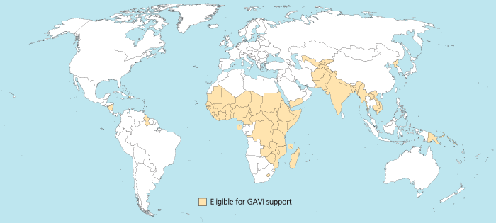
I was trying to reproduce the map of the GAVI Alliance eligible countries (btw I was surprised India is eligible – but that’s the beauty of relying on numbers only and not assumptions) in R. This is the original map (there are 57 countries eligible):

map_GAVI-eligible_countries_700x315_700

I started to use the R package rworldmap because it seemed the most appropriate for this task. Everything went fine. Most of the time was spent converting the list of countries from plain English to plain “ISO3” code as required (ISO3 is in fact ISO 3166-1 alpha-3). I took my source from Wikipedia.

Well, that was until joinCountryData2Map gave me this reply:

54 codes from your data successfully matched countries in the map
3 codes from your data failed to match with a country code in the map
189 codes from the map weren’t represented in your data

I should have better simply read the documentation: there is another small command that needs not to be overlooked, rwmGetISO3. What are the three codes that failed to match?

Although you can compare visually the map produced with the map above, R (and rworldmap) can indirectly give you the culprits:

tC2 = matrix(c("Afghanistan", "Bangladesh", "Benin", "Burkina Faso", "Burundi", "Cambodia", "Cameroon", "Central African Republic", "Chad", "Comoros", "Congo, Dem Republic of", "Côte d'Ivoire", "Djibouti", "Eritrea", "Ethiopia", "Gambia", "Ghana", "Guinea", "Guinea Bissau", "Haiti", "India", "Kenya", "Korea, DPR", "Kyrgyz Republic", "Lao PDR", "Lesotho", "Liberia", "Madagascar", "Malawi", "Mali", "Mauritania", "Mozambique", "Myanmar", "Nepal", "Nicaragua", "Niger", "Nigeria", "Pakistan", "Papua New Guinea", "Rwanda", "São Tomé e Príncipe", "Senegal", "Sierra Leone", "Solomon Islands", "Somalia", "Republic of Sudan", "South Sudan", "Tajikistan", "Tanzania", "Timor Leste", "Togo", "Uganda", "Uzbekistan", "Viet Nam", "Yemen", "Zambia", "Zimbabwe"), nrow=57, ncol=1)
apply(tC2, 1, rwmGetISO3)

In the results, some countries are actually given in a slightly different way by GAVI than in R. For instance “Congo, Dem Republic of” should be changed for rworldmap in “Democratic Republic of the Congo” (ISO3 code: COD). Or “Côte d’Ivoire” should be changed for rworldmap in “Ivory Coast” (ISO3 code: CIV). An interesting resource for country names recognised by rworld map is the UN Countries or areas, codes and abbreviations. Once you correct this, you can have your map of GAVI-eligible countries:

GAVIcountries-eligibles-map3-jepoirrier

And here is the code:

# Displays map of GAVI countries
library(rworldmap)
theCountries <- c("AFG", "BGD", "BEN", "BFA", "BDI", "KHM", "CMR", "CAF", "TCD", "COM", "COD", "CIV", "DJI", "ERI", "ETH", "GMB", "GHA", "GIN", "GNB", "HTI", "IND", "KEN", "PRK", "KGZ", "LAO", "LSO", "LBR", "MDG", "MWI", "MLI", "MRT", "MOZ", "MMR", "NPL", "NIC", "NER", "NGA", "PAK", "PNG", "RWA", "STP", "SEN", "SLE", "SLB", "SOM", "SDN", "SSD", "TJK", "TZA", "TLS", "TGO", "UGA", "UZB", "VNM", "YEM", "ZMB", "ZWE")
GaviEligibleDF <- data.frame(country = c("AFG", "BGD", "BEN", "BFA", "BDI", "KHM", "CMR", "CAF", "TCD", "COM", "COD", "CIV", "DJI", "ERI", "ETH", "GMB", "GHA", "GIN", "GNB", "HTI", "IND", "KEN", "PRK", "KGZ", "LAO", "LSO", "LBR", "MDG", "MWI", "MLI", "MRT", "MOZ", "MMR", "NPL", "NIC", "NER", "NGA", "PAK", "PNG", "RWA", "STP", "SEN", "SLE", "SLB", "SOM", "SDN", "SSD", "TJK", "TZA", "TLS", "TGO", "UGA", "UZB", "VNM", "YEM", "ZMB", "ZWE"),
GAVIeligible = c(1, 1, 1, 1, 1, 1, 1, 1, 1, 1, 1, 1, 1, 1, 1, 1, 1, 1, 1, 1, 1, 1, 1, 1, 1, 1, 1, 1, 1, 1, 1, 1, 1, 1, 1, 1, 1, 1, 1, 1, 1, 1, 1, 1, 1, 1, 1, 1, 1, 1, 1, 1, 1, 1, 1, 1, 1))
GAVIeligibleMap <- joinCountryData2Map(GaviEligibleDF, joinCode = "ISO3", nameJoinColumn = "country") mapCountryData(GAVIeligibleMap, nameColumnToPlot="GAVIeligible", catMethod = "categorical", missingCountryCol = gray(.8))

Visualizing categorical data in mosaic with R

A few posts ago I wrote about my discomfort about stacked bar graphs and the fact I prefer to use simple table with gradients as background. My only regret then was that the table was built in a spreadsheet. I would have liked to keep the data as it is but also have a nice representation of these categorical data.

This evening I spent some time analysing results from a survey and took the opportunity to buid these representations in R.

The exact topic of the survey doesn’t matter here. Let just say it was a survey about opinion and recommendations on some people. The two questions were:

  1. How do you think these persons were, last year? Possible answers were: very bad, bad, average, good or very good.
  2. Would you recommend these persons for next year? Possible answers were just yes or no.

For the first question, the data was collected in a text file according to these three fields: Person, Opinion, Count. Data was similar to this:

Person,Opinion,Count
Person 1,Very bad,0
Person 1,Bad,0
Person 1,Average,4
Person 1,Good,9
Person 1,Very good,3
Person 2,Very bad,3
Person 2,Bad,4
Person 2,Average,4
Person 2,Good,5
Person 2,Very good,0

The trick to represent this is to use  geom_tiles (from ggplot2) to display each count. There is an additional work to be done in order to have the Opinion categories in the right order. The code is the following:

library(ggplot2)
data1 <- read.table("resultsQ1.txt", header=T, sep=",")
scale_count <- c("Very bad", "Bad", "Average", "Good", "Very good")
scale_rep <- c("1", "2", "3", "4", "5")
names(scale_count) <- scale_rep
ggplot(data1, aes(x=Opinion, y=Person)) +
geom_tile(aes(fill=Count)) +
xlim(scale_count) +
scale_fill_gradient(low="white", high="blue")+theme_bw() +
opts(title = "Opinion on persons")

And the graph looks like this:

For the second question, the data was collected in a text file according to these three fields too: Person, Reco, Count. Data was similar to this:

Person,Reco,Count
Person 1,Recommend,16
Person 1,Do not recommend,0
Person 2,Recommend,5
Person 2,Do not recommend,11

And we use approximately the same code:

library(ggplot2)
data2 <- read.table("resultsQ2.txt", header=T, sep=",")
ggplot(data2, aes(x=Reco, y=Person)) +
geom_tile(aes(fill=Count)) +
scale_fill_gradient(low="white", high="darkblue")+theme_bw() +
opts(title = "Recommendations")

And the graph for the second question looks like this:

Easy isn’t it? Do you have other types of visualization for this kind of data?

R and the proxy server

R is a “a free software environment for statistical computing and graphics“. Being a desktop software, R is working out-of-the-box, even if you don’t have a network connection. However, if you want to install packages using a repository on the internet, you need a network connection (of course). If your computer happens to be behind a proxy server, you have to slightly modify your shortcut (in MS-Windows) to allow R to download packages. This can be done by modifying the “Target” field in the “Shortcut” tab of the shortcut properties (right-click on the shortcut to R, select tab “Shortcut”, edit field “Target”):

"C:\Program Files\R\R-2.12.2\bin\i386\Rgui.exe" http_proxy=http://proxyaddress:80 http_proxy_user=ask

Adapt the path to your R version, change the string “proxyaddress” by your proxy (see this previous post for a tip on this) and you’re done!

Because I never remember them, I’ll conclude this post with standard commands related to the installation of a packages:

Installing packages in R:
> install.packages("packageName", repos = "http://cran.ma.imperial.ac.uk/", dependencies = TRUE)

Notes:

  • You might get a window asking you for your firewall credentials and to choose a mirror server
  • CRAN repositories can be found here: http://cran.r-project.org/
  • This will download and install the package again, even if it is already installed

Updating packages in R:
> update.packages("deSolve") # for the deSolve package, for example

Know all packages installed in R on your computer:
> libraries()

Finally, here is a R reference card that can be useful too.